Quantitative Leveraged ETF Strategy

MFAM's Quantitative Leveraged ETF Strategy is a fully rules-based trading system combining three complementary quantitative engines, trend-following on the long side, mean reversion, and trend-following on the short side, across a basket of leveraged US and Chinese equity ETFs. Every entry, exit, and position size is driven by mathematical rules. There is no discretionary override.

Historical Performance

The strategy has been run against historical market data covering May 2017 through end-2024. From the start of 2025 onward the strategy has been running forward out-of-sample, with results accumulating on the same rules and all parameters frozen. Over the combined period the equity curve has meaningfully outpaced a passive S&P 500 investment.

MFAM Quantitative Leveraged ETF Strategy versus S&P 500 total return. Growth of $100k invested May 2017. The in-sample build window was 2019 to 2022. Pre-build data (May 2017 to end-2018) was held out as a backward out-of-sample test, never seen during the build. The 2023 to 2024 window was held out as a forward out-of-sample test and was where the risk-sizing parameters were recalibrated for three-times leverage. From the start of 2025 onward the strategy is running forward out-of-sample with all parameters frozen.

The strategy outperformed the benchmark in 10 of 10 calendar years. Outperformance years averaged roughly +34 percentage points above SPY. The asymmetry reflects the system's design preference for capturing large directional moves rather than tracking the benchmark closely.

Calendar-year returns side by side. The strategy outperformed SPY in 10 of 10 years. Outperformance years averaged +34 percentage points above SPY.

Context for this period

Long-run S&P 500 returns sit somewhere in the 7 to 10 per cent range depending on the period measured, averaging around 10 per cent in nominal terms over the past century. That average is made up of decades that look very different from each other, including the 1929-32 crash, the 1968-82 stagflation decade, the 2000-02 dot-com bust and the 2008 global financial crisis.

The May 2017 to April 2026 window has not looked like those decades. It has instead been one of the strongest stretches the benchmark has ever had, with a 14.8 per cent annualised return driven by uninterrupted tech-led leadership, fast recoveries from the 2020 COVID shock and the 2022 inflation shock, and an artificial-intelligence-driven capex cycle from 2023 onward. The benchmark is running well above its long-run average and sets a high bar.

The strategy outperformed that elevated benchmark by a meaningful margin. Historically, the strategy's edge has been largest in years with strong directional moves in either direction, including the 2017 and 2019 tech-led bull runs, the 2021 reopening, the 2024 AI-led extension, and notably 2022 where the trend-short engine and mean-reversion engine produced positive returns through a year that took the S&P 500 down 18 per cent. The single underperformance year was 2018, where the February volatility spike and the Q4 sell-off produced a -5.1 per cent strategy result against -4.6 per cent for the benchmark, a half-percentage-point gap. The structural edge is expected to be at least as visible against a long-run benchmark closer to the 7 to 10 per cent average than it has been against the far stronger backdrop of the past decade.

No guarantee is made about future performance. The point is that the strategy has beaten a very hot benchmark. A cooler benchmark is historically where this type of system has had its best relative years.

Alpha vs Beta

The first number most investors look at is return. A 52.6 per cent annualised strategy looks objectively better than a 14.8 per cent benchmark. The raw comparison hides something important though, because not all returns are created equal. A strategy's return number has to be broken down into two very different components before it can be judged honestly.

Beta is market exposure

Beta is the portion of a strategy's return that comes from simply being in the market. If the S&P 500 goes up 10 per cent in a year, a fully invested portfolio that moves in lockstep with it will also go up roughly 10 per cent. Nothing clever happened. The market rose, and the investor was along for the ride. Anyone willing to press a single buy button on an index ETF can collect beta. It requires no analysis, no timing, and no discipline.

Critically, beta is not free. It comes with full participation in market losses. The same passive portfolio that captured the upside will sit through the full drawdown when the market falls. The investor has no defence against a bear market. They accept whatever path the market delivers, peaks and troughs alike.

Alpha is return that does not come from market exposure

Alpha is what is left over after the beta portion has been accounted for. It is the portion of return that reflects a genuine edge, whether from timing, selection, risk management, or all three. Alpha is what separates an active strategy from a passive one. When a strategy delivers return that cannot be explained by market exposure alone, and delivers it with risk characteristics that are measurably different from a passive market allocation, that is alpha.

The distinction matters because alpha and beta are valued very differently. Beta is effectively free, available for a fraction of a per cent in management fees through any index ETF. Alpha is scarce, because it requires a source of edge that most market participants do not have. Decades of academic and industry research confirm that consistent alpha is rare, and strategies that can demonstrate it are treated as materially different from strategies that simply ride the market higher.

How this strategy generates alpha

This strategy's outperformance versus the S&P 500 is not a function of taking more market risk. The opposite is true. Over the May 2017 to April 2026 window it produced a 52.6 per cent annualised return against 14.8 per cent for the S&P 500, while simultaneously containing its maximum drawdown to 29.5 per cent versus 33.7 per cent for the benchmark. Higher return and lower drawdown at the same time. That combination cannot be produced through beta alone. More market exposure would have produced deeper drawdowns, not shallower ones.

The strategy uses rules to pull capital out of the market when conditions no longer support its trading signals, and to deploy capital more aggressively when conditions do. A passive buy-and-hold investor has no mechanism to do either. They are always fully exposed regardless of whether the environment is favourable. The strategy's alpha comes from this selective exposure, applied mechanically by the rules rather than discretionarily by a human. The risk-adjusted metrics in the next section are where this alpha becomes visible, and the regime filter that drives the selective exposure is explained further down the page.

Risk-Adjusted Return Profile

Raw return alone understates the quality of the strategy. The cleanest way to judge a leveraged trading system is to compare its return per unit of worst-case drawdown taken to get there.

Risk-adjusted ratios — Calmar, Sharpe, Sortino — May 2017 through April 2026.

The Calmar ratio is the headline metric for this type of system. It divides the annualised return by the worst peak-to-trough drawdown across the period, which captures the question every leveraged-ETF investor should be asking, namely how much return was extracted for each unit of drawdown actually experienced. The strategy's Calmar of 1.78 is roughly four times the S&P 500's 0.44 over the same window. Headline CAGR is 52.6 per cent versus 14.8 per cent, and despite trading two- and three-times leveraged instruments the strategy's worst drawdown was -29.5 per cent against -33.7 per cent for the benchmark. The drawdown containment is what makes the higher CAGR meaningful, because a leveraged strategy that produced the same return through deeper drawdowns would not be the same product.

Sharpe and Sortino ratios are not the most useful metrics for this kind of system. Both measure variance around the mean, and a leveraged-ETF strategy is engineered to produce large positive moves on the days the underlying setups fire. Those large moves are exactly what the strategy exists to capture, and ratios that penalise them on a daily basis understate the quality of an outcome that is best judged on a peak-to-trough basis. The strategy's Sharpe ratio over the period was 1.226 and its Sortino was 1.321, both shown alongside Calmar in the chart above, but the headline question for a strategy of this design is whether the return justifies the worst drawdown taken, which is what the Calmar plus the drawdown chart together describe.

The mechanical source of the alpha is an intentional reduction in market exposure during adverse regimes, combined with an opportunistic short-side engine that profits when the long side is in cash. That regime-shifted exposure is what produces a higher return at a shallower drawdown, and is covered in the engine and regime filter sections below.

Why Maximum Drawdown Is the Number That Actually Matters

Most investors focus on return. Experienced investors focus on drawdown, because the arithmetic of recovery is unforgiving. A loss and a subsequent gain of the same percentage do not cancel out. The deeper the drawdown, the more disproportionate the recovery required.

A 50% drawdown requires a 100% gain to break even, which at historical equity market return rates takes roughly seven years. A 75% drawdown requires a fourfold return and realistically may never be recovered within an investor's remaining time horizon. Drawdown is not just a number on a chart. It is a direct tax on future compounding, and in severe cases it ends the compounding journey entirely.

The gap between the strategy's -29.5% maximum drawdown and the S&P 500's -33.7% may look modest at first glance, but the relevant comparison is not the headline drawdown number alone. The strategy delivered a 52.6 per cent annualised return for that drawdown, against a 14.8 per cent return for a benchmark that took an essentially identical drawdown. Per unit of worst-case drawdown experienced, the strategy compounded capital roughly three times faster. The Calmar ratio is the formal expression of that, and it is the metric that matters most for a leveraged-ETF system because it answers the question every drawdown-aware investor is asking, namely how much return was actually extracted for each unit of pain endured.

This is also why any strategy quoting strong headline returns should be scrutinised for the path it took to get there. Large returns achieved through large drawdowns are statistically fragile. The strategy here is engineered to contain the left tail first and let returns compound as a consequence, rather than the other way around.

Underwater drawdown curves measured from each series's running peak, May 2017 to April 2026.

Plotted continuously, the strategy's drawdown profile sits above the S&P 500's through most of the period. The worst trough was -29.5% versus -33.7% for the benchmark, and recovery back to new highs tends to happen faster. The 2020 COVID shock and the 2022 bear market are both visibly shallower and shorter for the strategy, which is the regime filter cutting exposure during adverse periods, and the trend-short engine taking over when long-side conditions deteriorate.

Historical Drawdown Events in Context

A feature of a leveraged-ETF strategy worth understanding is that its largest drawdowns tend to follow its largest rallies. The two- and three-times leveraged instruments produce outsized spikes during favourable regimes, and any subsequent consolidation is measured against that spike. The headline drawdown number reflects how much of a prior rally was given back, not how much base capital was put at risk.

A second, structural driver of these events is the trend engines' own design. Trend-following systems, on either the long or short side, are built to capture the bulk of a sustained move, not to exit at the top. The exit signal requires confirmation that the trend has weakened, which by construction occurs after the peak rather than at it. That confirmation requirement is precisely what allows the system to ride extended trends without being shaken out by mid-trend pullbacks. The cost of that patience is that a portion of the final leg of every trend is given back before the exit fires. This giving-back is not the strategy failing. It is the engine behaving exactly as designed, accepting a few percentage points of peak-to-exit slippage in exchange for the ability to hold winning positions through long, profitable runs. A trend system optimised to avoid give-back would also exit much earlier in its winners, sacrificing the tail of outlier returns that the long-tail distribution depends on.

Across May 2017 through April 2026 the strategy experienced six completed peak-to-trough drawdowns of 20% or more, with a seventh event currently in recovery. The cluster between -20.9% and -29.5% is consistent across regimes, which is the operating point the volatility-adjusted stops and per-leg risk caps are calibrated to enforce. No completed drawdown extended materially beyond the design envelope, and no event left the curve below an earlier trough by a meaningful margin. The strategy's all-time maximum drawdown of -29.5% sits inside event 4, the March 2022 rate-hike sell-off. Each red band on the chart marks one event with its peak-to-trough magnitude on the upper badge, and each green arrow marks the trough-to-new-high recovery that followed. The numbers below the chart correspond to the badges on each event.

Each red band marks a peak-to-trough drawdown of 20% or more, numbered chronologically. Seven events across the nine-year window — six completed and one in recovery — all sitting between -20.9% and -29.5%, with the deepest at -29.5% inside event 4. Green arrows mark the recovery gain from each trough to the next all-time high. This is the design operating range for the volatility-stop and per-leg risk-cap framework.

Each event follows the same pattern. A sustained rally produces a new all-time high, the underlying ETFs reach a regime inflection, and the strategy gives back a portion of the unrealised gain before the regime filter, the volatility-adjusted stops or the trend-short engine cut net exposure. Each drawdown is substantial in peak-to-trough terms, but the magnitude clusters in a tight band rather than running away to deeper levels. That tightness is the signature of a working risk-control framework.

1. 2018 Volmageddon and rolling 2018 sell-off (-27.8%, peak Jan 2018, trough Feb 2019, recovered Apr 2019). The February 2018 volatility spike, the Q4 2018 equity drawdown and the early-2019 trough rolled into one extended event lasting roughly thirteen months. Volatility-adjusted stops exited long positions through each leg as realised vol expanded. The strategy compounded +104% from this trough to its next all-time high in January 2020.
2. Q1 2020 COVID crash (-25.3%, peak Jan 2020, trough Feb 2020, recovered Jul 2020). An extremely rapid sell-off across global equities. The trough was reached in just six weeks. Volatility-adjusted stops exited losing positions and the trend-short engine took over as net exposure rotated. The strategy compounded +60% from this trough to its next all-time high in September 2020.
3. Q3 2020 post-COVID retrace (-20.9%, peak Sep 2020, trough Sep 2020, recovered Nov 2020). A sharp three-week consolidation through the September 2020 US election period after a multi-month rally. The October trough sat well above the April 2020 trough, illustrating the strategy compounding through cycles. The strategy compounded +227% from this trough to its next all-time high in March 2022.
4. 2022 rate-hike sell-off (-29.5%, peak Mar 2022, trough Apr 2022, recovered Aug 2022) — the all-time MDD. The first major leg of the Fed tightening cycle. This is the deepest drawdown in canon history and sits exactly at the design envelope. The trend-long engine moved to cash, the trend-short engine took over net exposure, and the book recovered to a new high inside five months. The strategy compounded +73% from this trough to its next all-time high in October 2022.
5. Late 2022 to early 2023 banking stress (-22.0%, peak Oct 2022, trough Mar 2023, recovered May 2023). A persistent grind down through the back half of 2022 and into the March 2023 Silicon Valley Bank failure and regional-bank stress episode. The directional engines rotated as macro regime signals shifted. The strategy compounded +243% from this trough to its next all-time high in May 2024 — the largest run-up in canon history.
6. Mid-2024 to late-2024 chop (-26.8%, peak May 2024, trough Nov 2024, recovered Apr 2025). A persistent rotation between mega-cap leadership and broader-market participation through US election year. The directional engines whipsawed before the trend-short engine and mean-reversion engine stabilised the book. The strategy compounded +121% from this trough to its next all-time high in October 2025.
7. Q4 2025 to Q1 2026 sell-off (-25.7%, peak Oct 2025, trough Mar 2026, recovery in progress). A two-stage sell-off driven by escalating Iran and Middle East conflict, renewed tariff and policy uncertainty, and a sharp momentum unwind through February and March 2026 where the S&P 500 fell 8.9% in four weeks and the underlying leveraged ETFs fell 33 to 43% peak to trough. Sits well within the design envelope and is the most recent of the seven events.

Frequent but Bounded — the Diversification Fingerprint

If the maximum drawdown number tells you how deep the worst event was, the drawdown profile tells you how the strategy actually feels to live with day to day. The picture below plots the strategy's drawdown against the S&P 500 over the same nine-year window.

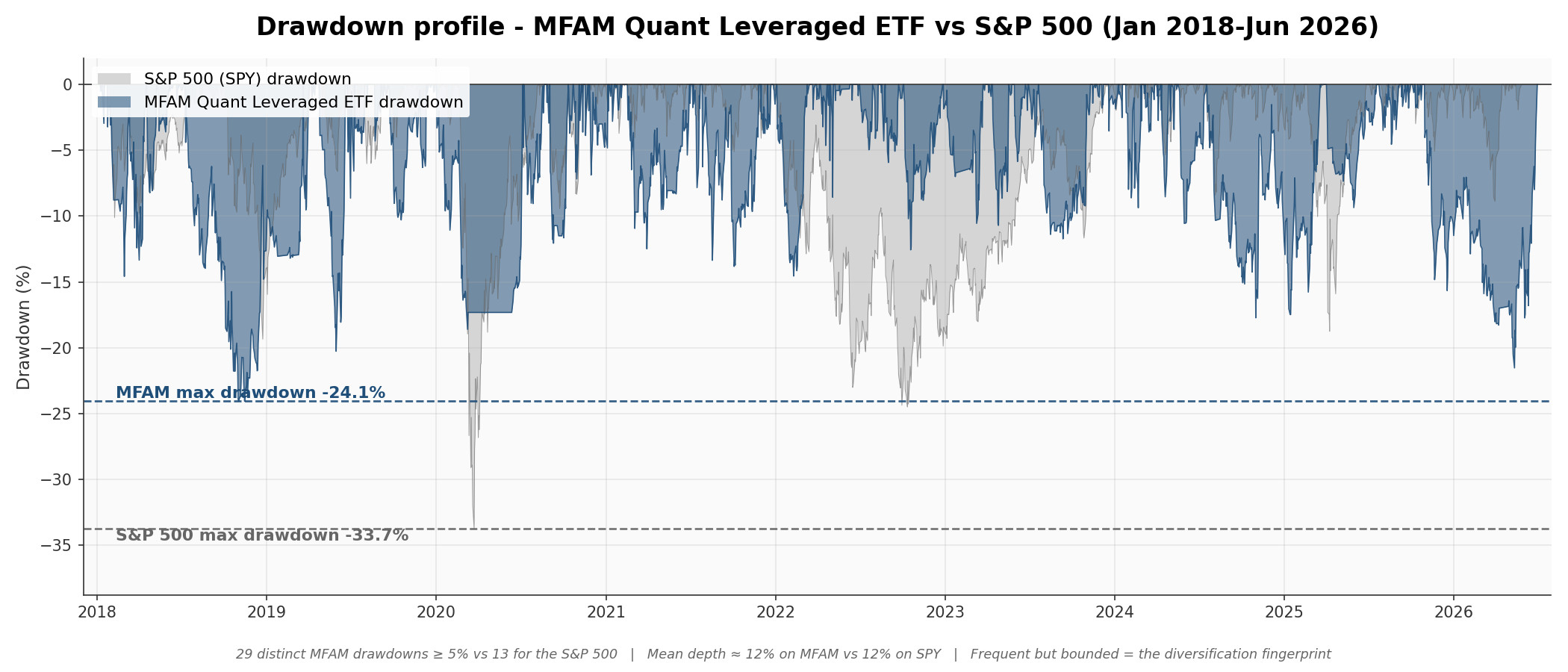
Two things stand out. First, the strategy is in some kind of drawdown roughly nine days out of every ten — there are thirty-two distinct drawdown events of five per cent or deeper across the window, against thirteen for the S&P 500. Second, despite that frequency, the deepest drawdown is shallower than the S&P's: -29.5 per cent versus -33.7 per cent.

That combination is the diversification fingerprint of the strategy. Thirteen leveraged instruments running across three engines means new local peaks are reached constantly, which means small recedes from those peaks happen constantly. The strategy is almost never sitting on an all-time high. But the same diversification means no single engine's bad month can drag the whole book past the design envelope of around thirty per cent. The drawdowns are frequent, but they are bounded.

This profile has a side-effect on the headline statistics. The strategy's Sharpe ratio of 1.226 is good but not extraordinary, because Sharpe penalises every move equally — including the large up days that drive the compounding. The Calmar ratio of 1.78, which only cares about how deep things ever got, is closer to four times the S&P's. The Calmar gap is the more honest read for a strategy of this design, because it captures the asymmetry: shallow drawdowns paired with hard up moves.

How It Works

The strategy runs three engines in parallel, each trading different signals across different instruments. The three engines are designed to work in different market regimes so that the strategy as a whole has exposure to trending up, trending down, and mean-reverting environments. The drawdown containment shown above is not an accident, it is the direct mechanical consequence of how the three engines are designed to switch leadership across regimes.

Trend-Long Engine

Identifies established uptrends using a combination of momentum indicators, moving-average filters, and a regime-detection layer. The engine stays out of the market when broader conditions do not support long-side trend-following. Exits are driven by volatility-adjusted trailing stops that tighten as a trade moves in favour.

Mean-Reversion Engine

Identifies short-term oversold conditions in volatile sectors and takes positions sized to capture rebounds. Exits again use volatility-adjusted stops, with discipline around capturing the first material reversion move rather than holding for extended trends.

Trend-Short Engine

The mirror image of the trend-long engine, applied to the inverse leveraged ETFs of the same underlying indices. It activates when sustained downtrends are confirmed by the regime layer, allowing the strategy to extract return from extended sell-offs rather than sitting in cash through them. Exits use the same volatility-adjusted stop framework as the trend-long engine.

Three Engines, Three Trade Profiles

The three engines produce very different trade shapes. The two trend engines are designed to catch extended directional moves and hold them through a sustained leg, which typically means multi-week to multi-month hold times. The mean-reversion engine is the opposite, entering after a short sharp dislocation and exiting as soon as price snaps back, often within a few days. The performance of the strategy is driven by the distribution of outcomes across hundreds of trades rather than any single winner.

How the Three Engines Switch Across Regimes

The three engines have substantially uncorrelated exposure patterns. When long-side trend conditions are poor, the regime filter pulls the trend-long engine into cash. When short-side trend conditions activate, the trend-short engine takes over net exposure. The mean-reversion engine fills in when neither trend regime is dominant. In practice, leadership rotates depending on what the market is doing.

Average fraction of each engine's legs held during the year, 2017 to 2026.

The 2018 Q4 sell-off and the 2022 rate-hike bear are the clearest illustrations. The trend-long engine was held in cash for extended periods through both, while the trend-short engine carried directional exposure on the way down and the mean-reversion engine captured the intervening relief rallies. In strongly trending bull years such as 2019, 2021 and 2024, the trend-long and mean-reversion engines run concurrently at high exposure while the trend-short engine sits in cash.

The mechanical consequence of this rotation is that the strategy is rarely flat across all three engines, and is also rarely fully exposed across all three at the same time. Net market exposure adapts to the current regime rather than running at a fixed level. This is the structural reason the strategy's maximum drawdown over the historical period was -29.5% versus -33.7% for the S&P 500, despite trading two- and three-times leveraged instruments. The regime filter and the trend-short engine together remove or reverse capital exposure when the environment does not support the long-side signal. Drawdown containment, and the alpha that comes with it, follows as a side effect of that discipline.

Proprietary Signal Calibration

All three engines use a proprietary approach to signal tuning, allowing faster regime detection than conventional moving-average or crossover methodologies. This responsiveness is a core part of the edge and comes from extensive quantitative research rather than any single technical indicator.

For a plain-language walkthrough of the trend, mean-reversion, regime-filter and volatility-stop concepts this strategy is built on, access the free MFAM trading course.

Instrument Selection

The strategy trades thirteen leveraged exchange-traded funds, five on each trend engine and three on the mean-reversion engine. Instrument selection is deliberate and follows three principles. The first is that each instrument must sit in a market segment whose behaviour matches the engine trading it. Trend legs are placed in markets with a history of long, persistent directional moves. Mean-reversion legs are placed in sectors where sharp dislocations reliably snap back. The second principle is non-overlapping exposure. Each leg tracks a distinct sector or geography, so an adverse event in one does not cascade across the book. The third is liquidity. Every instrument is a top-tier ETF with deep order books, so fills are reliable and position sizing is not constrained.

Leverage is used intentionally. The two- and three-times-leveraged structure amplifies every signal, allowing the system to extract meaningful return from moves that would be uneconomic to trade in unleveraged form. The same leverage is what makes stop-loss discipline and regime filtering non-negotiable, and the strategy is engineered around that requirement.

Trend-Long Engine Instruments

Mean-Reversion Engine Instruments

Trend-Short Engine Instruments

Every Trade Matters

Quantitative strategies rely on statistical discipline. The distribution of individual trade outcomes over the backtest period demonstrates why taking every signal, without filtering, is a structural requirement.

Distribution of returns across 318 closed trades, May 2017 through April 2026.

Trade outcomes follow a long-tailed distribution. Most trades produce small positive or small negative returns, clustered near the mean, with a long right tail of outsized winners. The win rate across the period was approximately 54 per cent.

Equally important is what happens on the left-hand side of the distribution. Most losing trades sit between zero and minus ten per cent, and the ten worst losses all sat between -26 and -42 per cent on the underlying leveraged ETF. None of the ten worst trades exceeded the -42 per cent floor that the volatility-stop and per-leg risk-cap framework is engineered to enforce. There is no single catastrophic blow-up trade that unwound prior gains. The left side of the distribution is bounded by the risk-control framework rather than by chance.

Two risk controls produce this shape. The first is stop-loss discipline. Every position carries a volatility-adjusted stop that tightens as a trade moves in favour, so losing trades are exited mechanically at a pre-defined loss rather than allowed to deteriorate. The second is per-leg risk sizing, which targets a fixed dollar-risk budget per trade based on each instrument's recent realised volatility. High-volatility instruments receive smaller position sizes so that the dollar loss at the stop is consistent across the book. Combined, these two controls are what allow the strategy to run leveraged instruments without carrying catastrophic single-trade risk, and are the reason the left tail of the distribution stays bounded.

Is This Just Curve Fitting?

A fair question to ask of any backtested strategy is whether the performance is real or whether the rules have been retro-fitted to the data until the equity curve looks good. This is called curve fitting, and it is the single most common failure mode of quantitative research. A curve-fit strategy will show a beautiful historical track record and then fall apart the moment it is asked to trade on data it has not seen. The numbers on the chart were engineered into existence, not discovered.

Curve fitting is easy to do accidentally. Any strategy has parameters, and any parameter can be tuned until the historical result is maximised. If you try enough combinations on the same dataset, something will fit that dataset almost perfectly by coincidence alone. The fit says nothing about the future because the rules were selected for that specific history, not for any underlying market behaviour. A properly engineered quantitative strategy has to be built in a way that makes this kind of overfitting structurally difficult.

How to tell curve fitting from a real edge

The cleanest test is a parameter sweep. Take the finished strategy, vary its core parameters over a wide range, and plot every resulting equity curve. If the strategy's performance collapses when the parameters move even slightly, the historical result was a lucky coincidence at one specific parameter setting. If the curves instead form a tight cluster, with every variant producing similar shape and similar ending value, the edge lives in the underlying rules, not in the specific numbers chosen. The parameter sweeps shown below were generated on the original six-leg development build of the strategy, which contains the trend-long and mean-reversion engines tested in isolation before the trend-short engine and the additional leveraged ETFs were folded into the deployed configuration. They are shown to demonstrate parameter-stability methodology and are not intended to reproduce the headline performance figures above, which are calculated on the full thirteen-leg deployed configuration.

A well-built strategy has to be robust on both sides of every trade, the entry and the exit. Sweeping only one side leaves the other side unexamined. Both sides are tested independently below.

Exit-side robustness, the volatility-stop sweep

The exit side of the strategy is governed by volatility-adjusted stops. Each position is given a stop whose distance scales with how noisy the underlying instrument currently is, so a calm market produces tight stops and a noisy market produces wider ones. The question is whether the edge depends on the specific stop multiples chosen, or whether it holds across a range of reasonable values.

Volatility Stop Parameter Sweep. Twenty-five equity curves produced by varying the trend-engine and mean-reversion exit-stop multipliers across a wide range of reasonable values, with the deployed configuration centred in the grid. Bold navy line is the deployed configuration. Green dashed line is the S&P 500. Generated on the six-leg development build of the strategy (trend-long plus mean-reversion engines, prior to the addition of the trend-short engine and the further leveraged ETFs in the deployed thirteen-leg configuration). Shown to illustrate parameter-stability methodology, not to reproduce the headline performance figures.

Every one of the twenty-five exit-parameter combinations beats the S&P 500 by a meaningful margin, and every curve follows the same overall shape through every drawdown and recovery. The cluster is tight, with ending values sitting in a narrow band relative to the total compounded return. There is no single knife-edge volatility-stop setting propping up the result. The exit logic works across the full plausible parameter space.

Entry-side robustness, the signal-length sweep

The entry side of the strategy is governed by lookback-window signals on each engine. Each signal has a lookback window that controls how sensitive it is. A shorter window produces more entries and more noise. A longer window produces fewer entries but waits for more confirmation. The second sweep varies the trend and mean-reversion lookbacks independently to test whether the edge survives different signal sensitivities.

Entry Signal Parameter Sweep. Twenty-five equity curves produced by varying the trend-engine and mean-reversion entry-signal lookback windows across a wide range of reasonable values, with the deployed configuration centred in the grid. Bold navy line is the deployed configuration. Green dashed line is the S&P 500. Generated on the six-leg development build of the strategy (trend-long plus mean-reversion engines, prior to the addition of the trend-short engine and the further leveraged ETFs in the deployed thirteen-leg configuration). Shown to illustrate parameter-stability methodology, not to reproduce the headline performance figures.

Again, every combination beats the benchmark by a meaningful margin and every curve retains the same overall path. The entry logic is not hanging on one specific lookback value. Whether the lookback windows are shorter or longer than the deployed configuration, the strategy still produces a similarly shaped equity curve ending materially above the S&P 500. Entry and exit are independently robust, which is the stronger test because it rules out the possibility that one side of the system is carrying the other.

Plateau selection, why the deployed setting is not the peak

A common and valid question when looking at a parameter grid is whether the deployed configuration was simply picked as the highest-performing cell. If the development process had done that, the deployed setting would be sitting at the top of a narrow spike, and any small move away from it would collapse performance. That is the curve-fitting failure mode a sweep is designed to detect.

The selection method used here was different. The grid was inspected across multiple planes, with return stability and drawdown stability both weighing equally into the decision. The goal was not to find the single best cell on any one metric. It was to find a cell whose neighbours produced similar returns and similar drawdowns, so that a small parameter miscalibration in deployed trading would not change the character of the results. Both planes were considered together, and the deployed setting was chosen from the region where the neighbourhood was consistent on both.

The heatmap below shows the profit factor plane of the same 5 by 5 entry-parameter grid, with the actual parameter values anonymised as x and y. Profit factor is the ratio of gross profits to gross losses, so any cell above 1.0 is net profitable. It is the cleanest way to visualise whether the edge survives away from the deployed configuration.

Profit factor across the 5 by 5 entry-parameter neighbourhood. Axis values are anonymised as x and y. The deployed configuration sits at the grid centre and is marked with a star. Green cells are higher profit factor; red would indicate breakeven.

The key feature is that every cell in the neighbourhood is green. Profit factor ranges from roughly 1.45 to 1.59 across the entire grid. A curve-fit strategy would show one green cell surrounded by red, with profitability collapsing as soon as any parameter moved. Instead, the whole neighbourhood is comfortably profitable. The edge is not sitting on a knife-edge parameter choice, it is being generated by the underlying rules and survives in every direction around the deployed setting.

The same broad stability shows up on the max-drawdown plane when it is inspected alongside this one. Drawdown is not uniform across the whole grid, but it clusters tightly in the region the deployed configuration was picked from, which is why both planes were weighed together at selection time rather than either one in isolation.

How the strategy was developed

The development process itself was designed to resist curve fitting, in three deliberate stages.

Stage one was building the base logic on unleveraged instruments. The trend and mean-reversion engines were designed and tested against one-times ETFs tracking the same underlying exposures, where signal behaviour is cleaner and leverage-related decay does not distort the data. The goal in this stage was to establish whether the underlying trading rules captured real market behaviour, independent of any amplification. If the rules did not work on the unleveraged instruments, they were not going to work anywhere.

Stage two was validation on data the rules had never seen, using both a backward and a forward out-of-sample test. The engines were built and their parameters chosen on the 2019 to 2022 window. Once the base logic performed on that development set, it was tested in two directions. Going backwards, the rules were run against the May 2017 to end-2018 window, which predates the build window and had never been seen during development. Going forwards, the rules were run against the 2023 to 2024 window, which had been deliberately held out of the build. If the rules had been curve-fit to the development data, performance on either out-of-sample window would have fallen apart. It did not, which is what gave confidence that the edge was structural rather than accidental.

Stage three was calibrating for the two- and three-times leveraged instruments actually deployed. Leverage changes the risk profile materially. During the 2023 to 2024 forward out-of-sample window, the volatility-stop multiples and regime-filter thresholds were re-tuned to accommodate the faster, larger moves that leveraged ETFs produce. This calibration did not change the underlying logic. It adjusted the risk-taking envelope so the same rules would operate safely on instruments that amplify every move by a factor of two or three. The rules themselves were not refit to the 2023 to 2024 data, only the risk-sizing parameters were recalibrated for leverage.

This staged process is why both parameter sweeps fan out tightly rather than collapsing when the parameters are varied. The underlying logic was validated before leverage-specific tuning was applied, so the strategy is not reliant on any specific choice of entry length or stop multiplier for its edge.

Current Status

Performance figures on this page are a combination of two periods. The May 2017 to end-2024 portion is historical simulation constructed from actual market data using the strategy's current rules. The 2025 portion onward is the strategy running forward out-of-sample, with results accumulating on the same rules and all parameters frozen. Both segments are shown continuously on the same equity curve, with a marker indicating the boundary between the historical-simulation and forward-out-of-sample periods.

How You Access the Strategy

The strategy is delivered as non-discretionary general advice. MFAM generates the signals and, once the investor authorises each one, the MFAM adviser places the order on the investor's behalf. The mechanics below are how that works in practice.

Your account, your custody

The investor opens their own account at Interactive Brokers. The account and all cash deposits are legally held by the investor, with client cash sitting in Interactive Brokers' segregated trust account under Australian and United States client-money rules. MFAM does not hold, pool, or control investor funds at any point. The account is yours, the money is yours, and you can close the account or withdraw at any time without MFAM's involvement. The MFAM adviser is added to the account as an authorised adviser with trading authority only, so orders can be placed on the investor's behalf once authorised, but cash cannot be moved out of the account by MFAM.

Signal delivery

General advice trade signals are issued to the investor by email and SMS during the trading day as the rules fire. Each signal is a specific instruction, the instrument, the side, and the size expressed as a percentage of portfolio. The investor only needs to reply yes to authorise. No action from the investor means no trade.

Execution

Once the investor has authorised a signal, the MFAM adviser places the order on the Interactive Brokers account. Orders are typically placed as market-on-open for the next United States session, which executes overnight Australian time. This matches how the strategy has been modelled, so executed orders track the backtest assumptions rather than drifting away from them.

Non-discretionary by design

Every trade requires explicit authorisation from the investor before it is placed. The MFAM adviser does not have discretion to enter or exit positions without a yes from the investor. This is general advice with client-authorised execution, not a managed account and not a managed fund. The investor decides whether any given signal is actioned, and can decline a signal or exit a position at any time.

Risk level is fixed, exposure scales with investment amount

The thirteen instruments used are a mix of two- and three-times leveraged ETFs, and the strategy's risk profile is fixed by its design rather than chosen by the investor. Volatility-adjusted dollar-risk parity sizing, a per-leg ceiling, and the adaptive slot count across the thirteen legs together define one risk profile that every investor receives, and that is the configuration the performance figures on this page are based on. The only dial the investor controls is how much capital to allocate to the strategy. A larger allocation produces a larger absolute swing in dollar terms, while the percentage return profile, drawdown profile, and per-leg risk budget remain the same regardless of investment size.

Cash-account structure, no broker margin

The strategy is engineered to run on an unmargined cash account. The investor's broker account holds the cash and the long ETF positions outright. There is no broker margin in use, no overnight financing or borrow cost, and no margin-call mechanic. The maximum loss on any individual trade is bounded by the position size and the volatility-stop, not by a forced-liquidation cascade triggered by a margin requirement.

The leverage that appears in the return profile comes from inside the underlying ETFs themselves. Direxion and similar issuers manage the daily rebalancing within each fund, and the investor pays for that operational service through the fund's expense ratio rather than through any borrow charge on their own account. This structure removes a class of failure mode — the gap-down forced-liquidation that ends careers in conventional margin-leveraged trading — and is the reason a strategy of this return profile can be run on a standard SMSF or retail brokerage cash account without margin-derived blow-up risk. Position-level losses on the underlying leveraged ETFs themselves remain real and material, and are managed by the strategy's volatility-stop and per-leg risk-cap framework.

Minimum investment

The strategy is offered from a minimum investment of AUD 20,000. There is no per-trade dollar minimum and no fixed monthly or platform fee. The all-in 30 basis-point per-fill charge applies on every entry and exit regardless of trade size, which works out to roughly 5 per cent per annum at the strategy's natural turnover. On a AUD 20,000 account that is approximately AUD 1,000 in annual fees, which the historical return profile is engineered to absorb. Fee specifics are discussed during the onboarding conversation with an MFAM adviser.